An Exploration and Explanation of Randomized Parameter Optimization
We’ve talked in the past about the importance of proper data when it comes to training a machine learning model, and how it is by far the most critical component when it comes to the accuracy and reliability of future results. However, we would be remiss to leave one with the idea that data alone is the be-all-end-all of a good model. While the importance of a good dataset cannot be overstated, the parameters behind the training of the model itself are also important variables in their own right and must be properly tuned if one wants their model to be the best it can be. However, the number of parameters any given model provides for the user to edit, what aspects of the model they affect, the ranges of input they take, and their relative importance all vary greatly between machine learning algorithms, and while many of them are able to be left on their default values and ignored, eventually a researcher will find themselves in a situation where they will be forced to come to grips with the multitude of options they have for what they want their final model to look like.
Obviously, such a task is beyond the capacity of your average human. With some algorithms having well over 20 parameters (many of which take choices from a continuous range of infinite values), and with the fact that the final impact of not just individual choices but their interactions can change results so drastically, it simply is not possible to find the optimal parameter choices given certain data by trial and error alone. Fortunately, with the aid of grid search, this problem, while maybe not perfectly solvable, can be solved enough for all practical purposes.
The most basic grid search algorithm is fairly straightforward: after passing it a training algorithm along with arrays of values for each parameter, it automatically goes through those arrays, training a model on each possible combination of those given parameter values, and selecting the one with the best result based on a score (such as its accuracy.) This alone, however, is still insufficient. Not only does this method take exponentially longer for models with more parameters (and as the arrays it chooses from for those parameters grow larger), selecting the values to go in those arrays is itself a similar problem to the one we try to avoid by doing grid search in the first place: it still requires a human being to figure out exactly what values should go in those arrays, based on either domain knowledge or trial and error. In fact, in some ways, it complicates that process further than if one was just asked to tune each parameter manually. In order to solve this, we need to move beyond simple arrays of discrete values: in order to decide continuous variables, we need to use continuous distributions.
Randomized grid search is one way to do this, removing the need for a person to determine which values should be included in the array for a given parameter by allowing them to submit a continuous distribution between two values instead. Of course, as such distributions are usually either infinite or practically infinite, it’s not a simple matter of iteration: such a grid search must involve random sampling, and it must be a sampling of a kind that takes into account matters such as training time and how many models it’s practically able to train. This does, however, narrow the things that a human needs to worry about from a large number of parameters and the arrays to choose for them from before to the much narrower question of what kind of temporal and processing budget one is comfortable with. Such a process can still take a large amount of such resources, however, and requires one final bit of refinement to make it more practical, through a process known as successive halving.
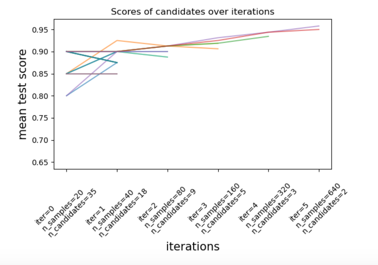
Basically, rather than training an entirely new model for each of randomly selected parameter permutations, the grid search algorithm starts out by dividing up a given dataset into a number of portions equal to a given number of models with randomly generated parameters (based off of the given distributions for each parameter.) This allows said models to be trained far faster than they would be if they were expected to use the full dataset. Then, after evaluation, the worst 50% of the models are dumped, with the samples they were trained on assigned to the remaining half. This continues until a final “victor” is reached, which is trained on the full dataset. In this way, the best parameters are able to be narrowed down in a fraction of the time it would take to train each model on the full dataset independently!
All of this having been done, we’re finally able to see which parameters are best for each model, without having had to try out an endless number of permutations manually and individually. And, as developments in ML continue, we might find our process getting even more streamlined in the future!