As we’ve discussed in our previous two Ex Machina articles, one of the goals in our machine learning efforts is to use artificial intuition as an aid in the construction of our signatures. This was previously illustrated by examining the importance of features in GB and RF algorithms, both of which are supervised techniques. However, both also require a training data set, which must be collected, annotated, and put together by humans; they’re good for finding patterns related to good or bad macros as a whole, but don’t get much more fine-grained than that. Obviously, this is going to lead to very general signatures. Even with very large training sets, the smaller details behind why an ML process yielded a positive or negative result are lost within simpler heuristics. When it comes to designing more specific signatures tailored to locating different kinds of malware, these heuristics are not enough.
We need a way to divide these broad groups of good and bad macros into smaller ones, called “clusters” or “families,” from which we can design new signatures (and even run them through another supervised algorithm to get machine insights.) Unfortunately, cutting up the data like this isn’t possible with the methods we’ve previously examined for two big reasons: we don’t know how many categories we’re going to end up dividing everything into, and, even if we did, we would need some way of measuring incorrect responses by the algorithm so it can learn, requiring the rules that we’re trying to find in the first place! This is a job for unsupervised learning, a branch of classifiers designed to find patterns in unlabeled data.
No Supervision Required
When we talk about unsupervised learning, it’s usually in the context of clustering. By clumping together similar data points, we ideally have distinct clusters start to emerge, in which all associated data points have a lot in common and all disassociated ones are vastly different. It is then from these clusters that we can begin to intuit families. There are a myriad of ways we can achieve clustering with ML, such as hierarchical clustering, k-means, and DBSCAN, all of which have their own advantages and disadvantages. One of the biggest hurdles any clustering algorithm must be able to overcome for our purposes is speed; with the large data sets we utilize, many strategies become untenable.
Enter MinHash
One of the biggest problems involved with picking out shared or unshared traits between files is the sheer computational complexity of it all. A large dataset will have to be grouped by comparing each candidate against every other possible candidate. Combine this with a large feature set, (such as which words are present in a document,)and you can end up with sets of thousands of features being compared against thousands of other sets with thousands of features. It simply isn’t feasible.
Fortunately, there are a class of algorithms that are excellent in circumnavigating this problem, and they are known as Locality-sensitive hashing (LSH) algorithms. By converting feature sets to smaller hashes of a fixed length, it turns out we’re able to estimate document similarities in a much more efficient manner. Just like any of the techniques we use, LSH comes in many flavors, but our method of choice is known as MinHash.
There are several ways you can measure the similarity of two documents, but the one MinHash favors is the Jaccard similarity, or the number of features that two sets have in common divided by the total features in both sets. This results in a number somewhere in the range of 0 to 1, with 0 indicating no commonalities and 1 representing sets that are identical. Now, there are multiple ways to arrive at the Jaccard similarity that don’t involve all this addition and division, and MinHash exploits a convenient coincidence to drastically cut down on processing time.
By running all features through the same hash function, and then keeping the minimum hash out of all of them, the vast feature sets of each data point are reduced down to a single number. It turns out, through some twist of fate, that the likelihood of any two hashes being the same is exactly equal to the Jaccard similarity of the files they represent! All thats left is to add a few more random hash functions and take the average to help smooth everything out.
Step-by-Step
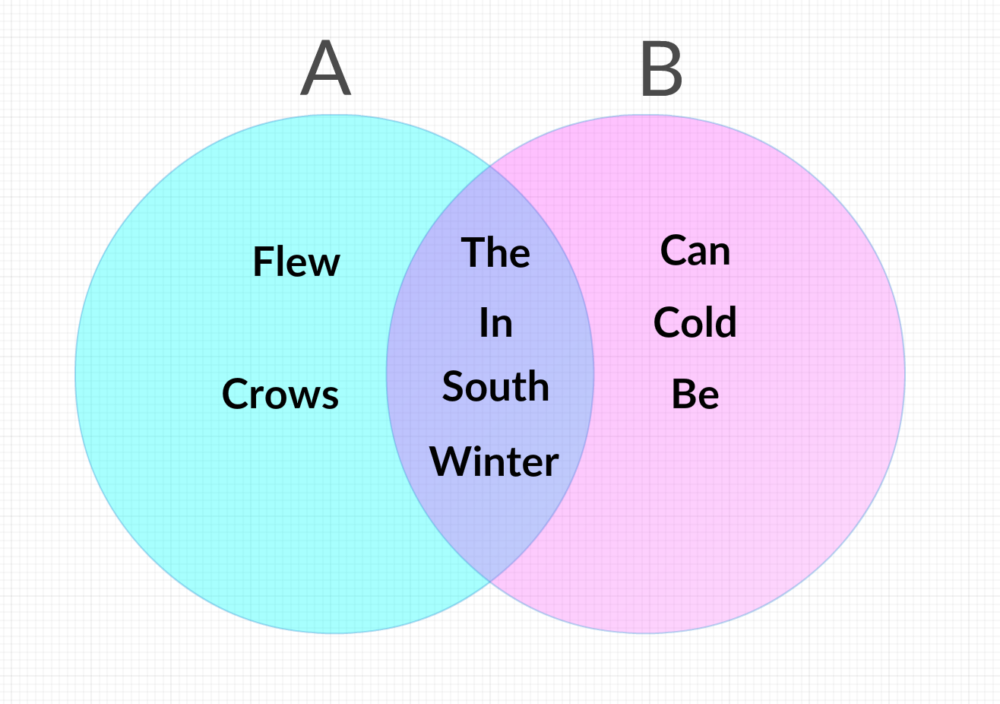
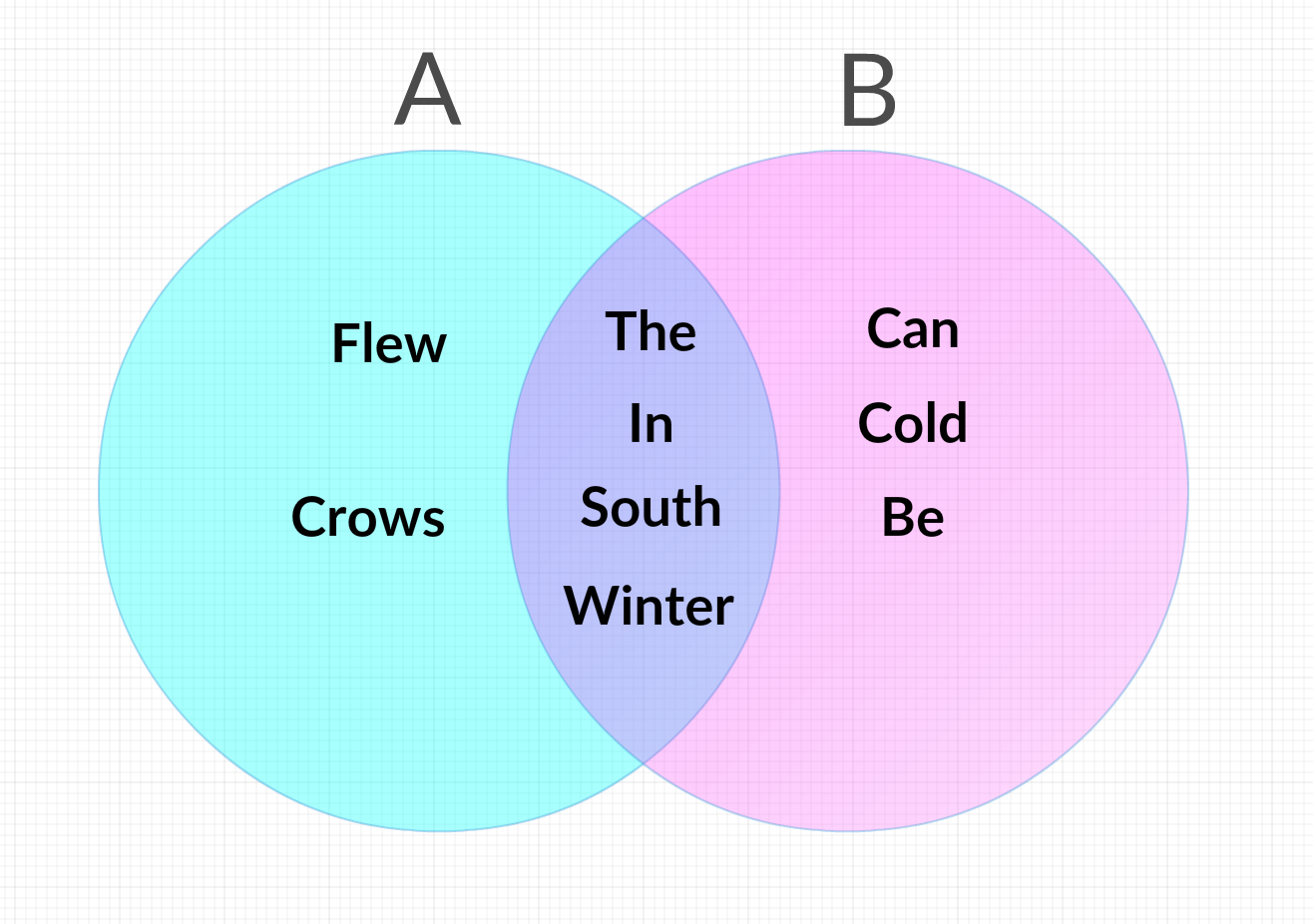
To make this a bit clearer, let’s walk through the comparison of two short, very simple documents, A and B. A contains nothing but the sentence “The crows flew south in the winter,” and B contains “In the south, winter can be cold.” We start out by simplifying them down by removing duplicate words within the same sentence.
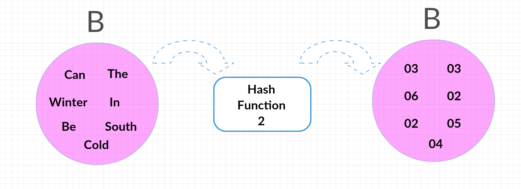
A becomes “The, crows, flew, south, in, winter” and B becomes “In, the, south, winter, can, be, cold.”
The Jaccard similarity of these two sets would then be the number of words they have in common, in this case 4, (south, the, in, and winter) divided by the total number of words, 9 (In, the, south, winter, can, be, cold, flew, and crow) to get 0.44.
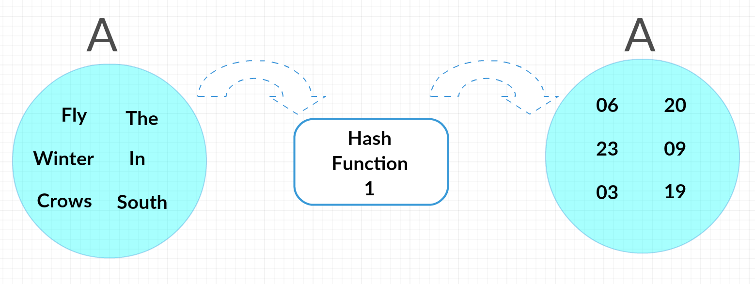
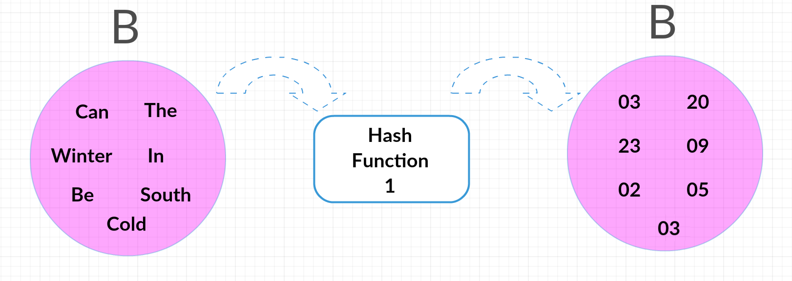
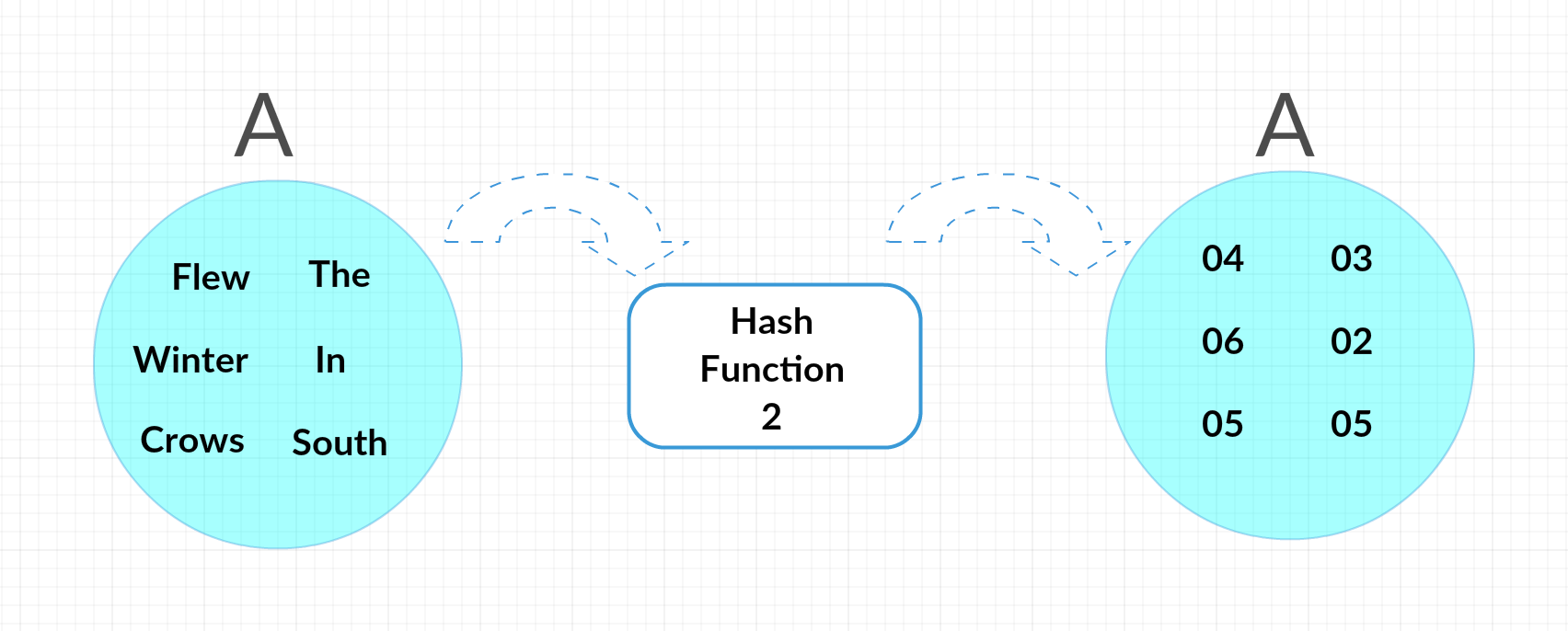
Now we can run these sets through multiple hash functions to get the average probability that they’ll wind up with the same end number. Our first hash function, for example, might be replacing each worth with the alphabetical index of its first letter, making A “03,20, 03, 06, 09, 23” and B “09, 20, 19, 23, 03, 02, 03” (notice how “cold” and “can” get assigned the same hash.) This leaves A with the smallest (minimum) has of 01, and B with 02. Not equal, but that’s okay; we’re going to need to do this with multiple hash functions to get the probability.
So, let’s say that for our second function we replace each word with its number of letters, making A “03, 05, 04, 05, 02, 06” and B “02, 03, 05, 06, 03, 02, 04.” This time the minimum hashes match; both are 02!
So we have two hash functions now, one that results in the documents not matching, and one that does. That would be a probability of 50%, and we can see we’re getting close to the true Jaccard. By repeating this processes with more and more hash functions, we begin to approach the true probability that any given hash will lead to identical numbers, and wind up with the Jaccard similarity without needing to compare each word in each sentence to each other word in the other one.
All that’s left is to set a threshold for what we consider “similar,” such as above 0.5, and clusters will begin to emerge, each made up of a group of documents above this threshold. Depending on how much overlap there is among clusters, it might be prudent to tweak the threshold a bit. The end result, though, is the data we started with, now automatically divided into separate, similar groups. Now we can finally examine those groups individually to see what they have in common, and use that information in the construction of future signatures.
Free On-Demand Webinar: Think Before You Click
Whether sent as an email attachment, sitting in your cloud or traversing the Web, file-borne threats have become a proven favorite for delivering malware and phishing campaigns. View our webinar on-demand and get firsthand tips about how to safeguard your cybersecurity stack with File Detection and Response (FDR) and stop file-borne threats in their tracks.
![]()